Because of its wide availability and relatively low learning curve compared to other data analysis tools like Power BI or Tableau, Excel remains one of the most popular software packages used by accountants, finance professionals and data scientists. So, for those of you who spend much of your workday inside Excel, I want to share a few of our favorite time-saving Excel tips and tricks to help you get more done in less time.
If you haven’t checked out our other blog post on Excel, now is a great time to catch up. The five Excel tips and tricks we share there are just as relevant as they were when I wrote them in 2017.
Now on to the Excel tips for today. Below is a list of the tips we will be covering. If there’s one in particular that interests you, just click the link to jump right to it.
- The Quickest and Easiest Way to Create Pivot Tables
- Select Large Amounts of Data without Scrolling
- Get Summary Data without Using Formulas
- Create Tables and Charts in Seconds
- Can’t Remember that Formula? Build It!
Excel Tips #1: The Quickest and Easiest Way to Create Pivot Tables
Especially when you are new to pivot tables or have a lot of complex data to work with, creating them can be a real hassle. Even if you’re a pivot table Pro wouldn’t you like to get your reporting done faster?
Excel is now smart enough to recommend pivot tables that fit your data. All you have to do is go to Insert | Pivot Tables, highlight the data you would like to include and choose the pivot table you like best. It’s that simple. Excel will now automatically create your table, which you can use to manipulate your data until your heart’s content. See how it works with the visual tutorial below.
Excel Tips #2: Select Large Amounts of Data without Scrolling
This one may seem simple, but it can really come in handy when you have a large amount of data in front of you. The easiest way to select an entire column in Excel is to select the first cell in that column or row and press Ctrl + Space bar. If you’d like to select a row instead of a column, highlight the first cell in the row and press Shift + Space bar
Note: this also works for selecting multiple rows and columns. Select the first cell in each of the rows or columns you’re interested in and use the keyboard commands I described above.
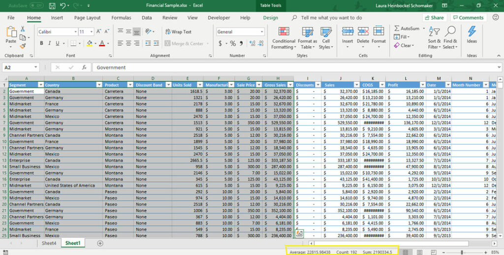
Excel Tips #3: Get Summary Data without Using Formulas
Once you’ve used the tip above to select the range of data you’re interested in, just look at the bottom of your screen. There you will find a variety of summary data like average, some and count, all calculated automatically for you without the need for any formulas.
Excel Tips #4: Create Tables and Charts in Seconds
This tip is another handy keyboard shortcut. Creating tables and charts in Excel is easy but takes several clicks. If you’re in a hurry to visualize your data with charts and tables, here’s the quickest way to do it.
To create a table, highlight the data you would like to include and press control + T on your keyboard. In an instant, a table will appear displaying your data. If you want to adjust the look of the automatically created table, all you have to do is select the table tab in the Excel ribbon and use the controls it offers to make any changes.
Creating a chart in a flash is very similar to the method I described for creating a table. This time, instead of pressing control + T, you’ll press Alt + F1. Again, if you want to make any adjustments to the chart that appears, you can do so by selecting the chart and using the design options that appear in the ribbon.
Excel Tips #5: Can’t Remember That Formula? Build It
The formulas available in Microsoft Excel give you endless options for data manipulation and calculation. However, unless you use the same formulas repeatedly, it’s difficult to remember the exact commands needed for a certain calculation.
So, with Excel 2016, Microsoft introduced the formula builder. This handy tool makes writing valid formulas, quicker and less frustrating than ever before. First, select the cell where you’d like the formula result to appear. Then, to open the formula builder, click the formulas tab on the ribbon, then “Insert Function.” A new dialog box will appear on the right side of your screen. If you cannot see the entire thing, or its location is inconvenient, just click it and drag it to a new spot on your screen.
Once you’ve got the dialog box where you want it, you will see it lists all available functions in Microsoft Excel. You can scroll through them to find the one you need or type the name of a function to bring it up. Clicking on the name of any function will display a short description. Use this information to decide if the function you selected is the one you need. Once you find the right one, click “Insert Function.”
Then, the formula builder will ask you what data you want to use in the formula. You can select the data in one of two ways. One, you can type the data in. Or, you can click the cells that contain the data you would like to use. My preferred method is to click the cells rather than type. This allows you to avoid typos or syntax errors. And if you accidentally click the wrong cell, all you have to do is choose the correct cell and Excel will update the formula for you.
If you’re unsure what information the function you’re working with requires, click on the “More help with this function” link at the bottom of the dialog box and a detailed explanation will appear. See how it works with the visual tutorial below.
There are our top five Excel tips for 2019. We hope these tips and tricks help you get more done in less time. Do you have a favorite Excel tip or trick you’d like to share? Leave it in the comments below.